It is important to know this relation because maps usually show the True Meridian and an observer is generally supplied with a magnetic compass. Fig. 15 shows the usual type of Box Compass. It has 4 cardinal points, N, E, S and W marked, as well as a circle graduated in degrees from zero to 360°, clockwise around the circle. To read the magnetic angle (called magnetic azimuth) of any point from the observer's position the north point of the compass circle is pointed toward the object and the angle indicated by the north end of the needle is read.
You now know from the meridians, for example, in going from York to Oxford (see Elementary Map) that you travel north; from Boling to Salem you must travel south; going from Salem to York requires you to travel west; and from York to Salem you travel east. Suppose you are in command of a patrol at York and are told to go to Salem by the most direct line across country. You look at your map and see that Salem is exactly east of York. Next you take out your field compass (Figure 15, Par. 1870), raise the lid, hold the box level, allow the needle to settle and see in what direction the north end of the needle points (it would point toward Oxford). You then know the direction of north from York, and you can turn your right and go due east towards Salem.
Having once discovered the direction of north on the ground, you can go to any point shown on your map without other assistance. If you stand at York, facing north and refer to your map, you need no guide to tell you that Salem lies directly to your right; Oxford straight in front of you; Boling in a direction about halfway between the directions of Salem and Oxford, and so on.
1871. Determination of positions of points on map. If the distance, height and direction of a point on a map are known with respect to any other point, then the position of the first point is fully determined.
The scale of the map enables us to determine the distance; the contours, the height; and the time meridian, the direction.
Thus (see map in pocket at back of book), Pope Hill (sm') is 800 yards from Grant Hill (um') (using graphical scale), and it is 30 feet higher than Grant Hill, since it is on contour 870 and Grant Hill is on contour 840; Pope Hill is also due north of Grant Hill, that is, the north and south line through Grant Hill passes through Pope Hill. Therefore, the position of Pope Hill is fully determined with respect to Grant Hill.
Orientation
1872. In order that directions on the map and on the ground shall correspond, it is necessary for the map to be oriented, that is, the true meridian of the map must lie in the same direction as the true meridian through the observer's position on the ground, which is only another way of saying that the lines that run north and south on the map must run in the same direction as the lines north and south on the ground. Every road, stream or other feature on the map will then run in the same direction as the road, stream or other feature itself on the ground, and all the objects shown on the map can be quickly identified and picked out on the ground.
Methods of Orienting a Map
1st. By magnetic needle: If the map has a magnetic meridian marked on it as is on the Leavenworth map (in pocket at back of book), place the sighting line, a-b, of the compass (Fig. 15) on the magnetic meridian of the map and move the map around horizontally until the north end of the needle points toward the north of its circle, whereupon the map is oriented. If there is a true meridian on the map, but not a magnetic meridian, one may be constructed as follows, if the magnetic declination is known:
(Figure 16): Place the true meridian of the map directly under the magnetic needle of the compass and then move the compass box until the needle reads an angle equal to the magnetic declination. A line in extension of the sighting line a'-b' will be the magnetic-meridian. If the magnetic declination of the observer's position is not more than 4° or 5°, the orientation will be given closely enough for ordinary purposes by taking the true and magnetic meridians to be identical.
2d. If neither the magnetic nor the true meridian is on the map, but the observer's position on the ground is known: Move the map horizontally until the direction of some definite point on the ground is the same as its direction on the map; the map is then oriented. For example, suppose you are standing on the ground at 8, q k' (Fort Leaven worth Map), and can see the U. S. penitentiary off to the south. Hold the map in front of you and face toward the U. S. penitentiary, moving the map until the line joining 8 and the U. S. penitentiary (on the map) lies in the same direction as the line joining those two points on the ground. The map is now oriented.
Having learned to orient a map and to locate his position on the map, one should then practice moving over the ground and at the same time keeping his map oriented and noting each ground feature on the map as it is passed. This practice is of the greatest value in learning to read a map accurately and to estimate distances, directions and slopes correctly.
True Meridian
1873. The position of the true meridian may be found as follows (Fig. 17): Point the hour hand of a watch toward the sun; the line joining the pivot and the point midway between the hour hand and XII on the dial, will point toward the south; that is to say, if the observer stands so as to face the sun and the XII on the dial, he will be looking south. To point the hour hand exactly at the sun, stick a pin as at (a) Fig. 17 and bring the hour hand into the shadow. At night, a line drawn toward the north star from the observer's position is approximately a true meridian.
The line joining the "pointers" of the Great Bear or Dipper, prolonged about five times its length passes nearly through the North Star, which can be recognized by its brilliancy.
1874. Conventional Signs. In order that the person using a map may be able to tell what are roads, houses, woods, etc., each of these features are represented by particular signs, called conventional signs. In other words, conventional signs are certain marks or symbols shown on a map to designate physical features of the terrain. (See diagram, Par. 1875 Plate I and II.) On the Elementary Map the conventional signs are all labeled with the name of what they represent. By examining this map the student can quickly learn to distinguish the conventional signs of most of the ordinary features shown on maps. These conventional signs are usually graphical representations of the ground features they represent, and, therefore, can usually be recognized without explanation.
For example, the roads on the Elementary Map can be easily distinguished. They are represented by parallel lines (======). The student should be able to trace out the route of the Valley Pike, the Chester Pike, the County Road, and the direct road from Salem to Boling.
Private or farm lanes, and unimproved roads are represented by broken lines (= = = =). Such a road or lane can be seen running from the Barton farm to the Chester Pike. Another lane runs from the Mills farm to the same Pike. The small crossmarks on the road lines indicate barbed wire fences; the round circles indicate smooth wire; the small, connected ovals (as shown around the cemetery) indicate stone walls, and the zigzag lines (as shown one mile south of Boling) represent wooden fences.
Near the center of the map, by the Chester Pike, is an orchard. The small circles, regularly placed, give the idea of trees planted in regular rows. Each circle does not indicate a tree, but the area covered by the small circles does indicate accurately the area covered by the orchard on the ground.
Just southwest of Boling a large woods (Boling Woods) is shown. Other clumps of woods, of varying extent, are indicated on the map.
The course of Sandy Creek can be readily traced, and the arrows placed along it, indicate the direction in which it flows. Its steep banks are indicated by successive dashes, termed hachures. A few trees are shown strung along its banks. Baker's Pond receives its water from the little creek which rises in the small clump of timber just south of the pond, and the hachures along the northern end represent the steep banks of a dam. Meadow Creek flows northeast from the dam and then northwest toward Oxford, joining Woods Creek just south of that town. York Creek rises in the woods 11/4 miles north of York, and flows south through York. It has a west branch which rises in the valleys south of Twin Hills.
A railroad is shown running southeast from Oxford to Salem. The hachures, unconnected at their outer extremities, indicate the fills or embankments over which the track runs. Notice the fills or embankments on which the railroad runs just northwest of Salem; near the crossing of Sandy Creek; north of Baker's Pond; and where it approaches the outskirts of Oxford. The hachures, connected along their outer extremities, represent the cut through which the railroad passes. There is only one railroad cut shown on the Elementary Map—about one-quarter of a mile northeast of Baker's Pond—where it cuts through the northern extremity of the long range of hills, starting just east of York. The wagon roads pass through numerous cuts—west of Twin Hills, northern end of Sandy Ridge, southeastern end of Long Ridge, and so on. The small T's along the railroad and some of the wagon roads, indicate telegraph or telephone lines.
The conventional sign for a bridge is shown where the railroad crosses Sandy Creek on a trestle. Other bridges are shown at the points the wagon roads cross this creek. Houses or buildings are shown in Oxford, Salem, York and Boling. They are also shown in the case of a number of farms represented—Barton farm, Wells farm, Mason's, Brown's, Baker's and others. The houses shown in solid black are substantial structures of brick or stone; the buildings indicated by rectangular outlines are "out buildings," barns, sheds, etc.
Plates I and II give the Conventional Signs used on military maps and they should be thoroughly learned.
In hasty sketching, in order to save time, instead of using the regulation Conventional Signs, very often simply the outline of the object, such as a wood, a vineyard, a lake, etc., is indicated, with the name of the object written within the outline, thus:
Such means are used very frequently in rapid sketching, on account of the time that they save.
By reference to the map of Fort Leavenworth, the meaning of all its symbols is at once evident from the names printed thereon; for example, that of a city, woods, roads, streams, railroad, etc.; where no Conventional Sign is used on any area, it is to be understood that any growths thereon are not high enough to furnish any cover. As an exercise, pick out from the map the following conventional signs: Unimproved road, cemetery, railroad track, hedge, wire fence, orchard, streams, lake. The numbers on the various road crossings have no equivalent on the ground, but are placed on the maps to facilitate description of routes, etc. Often the numbers at road crossings on other maps denote the elevation of these points.
Visibility
1875. The problem of visibility is based on the relations of contours and map distances previously discussed, and includes such matters as the determination of whether a point can or can not be seen from another; whether a certain line of march is concealed from the enemy; whether a particular area is seen from a given point.
On account of the necessary inaccuracy of all maps it is impossible to determine exactly how much ground is visible from any given point—that is, if a correct reading of the map shows a certain point to be just barely visible, then it would be unsafe to say positively that on the ground this point could be seen or could not be seen. It is, however, of great importance for one to be able to determine at a glance, within about one contour interval, whether or not such and such a point is visible; or whether a given road is generally visible to a certain scout, etc. For this reason no effort is made to give an exact mathematical solution of problems in visibility further than would be useful in practical work with a map in the solution of map problems in patrolling.
In the solution of visibility problems, it is necessary that one
should thoroughly understand the meaning of profiles and their
construction. A profile is the line supposed to be cut from the
surface of the earth by an imaginary vertical (up and down) plane.
(See Fig. 21.) The representation of this line to scale on a sheet of
paper is also called a profile. Figure 21 shows a profile on the line
D—y (Figure 20) in which the horizontal scale is the same as that of
the map (Figure 20) and the vertical scale is 1 inch = 40 feet. It is
customary to draw a profile with a greater vertical than horizontal
scale in order to make the slopes on the profile appear to the eye as
they exist on the ground. Consequently, always note especially the
vertical scale in examining any profile; the horizontal scale is
usually that of the map from which the profile is taken.
A profile is constructed as follows: (Fig. 21): Draw a line D'—y' equal in length to D—y on the map. Lay off on this line from D' distances equal to the distances of the successive contours from D on the map. At each of these contour points erect a perpendicular equal to the elevation of this particular contour, as shown by the vertical scale (960, 940, 920, etc.) on the left. Join successively these verticals by a smooth curve, which is the required profile. Cross section paper with lines printed 1/10 inch apart horizontally and vertically simplifies the work of construction, by avoiding the necessity of laying off each individual distance.
1876. Visibility Problem. To determine whether an observer with his eye at D can see the bridge at XX (Figure 20). By examining the profile it is seen that an observer, with his eye at D, looking along the line D—XX, can see the ground as far as (a) from (a) to (b), is hidden from view by the ridge at (a); (b) to (c) is visible; (c) to (d) is hidden by the ridge at (c). By thus drawing the profiles, the visibility of any point from a given point may be determined. The work may be much shortened by drawing the profile of only the observer's position (D) of the point in question, and of the probable obstructing points (a) and (c). It is evidently unnecessary to construct the profile from D to x, because the slope being concave shows that it does not form an obstruction.
The above method of determining visibility by means of a profile is valuable practice for learning slopes of ground, and the forms of the ground corresponding to different contour spacings.
Visibility of Areas
1877. To determine the area visible from a given point the same method is used. First mark off as invisible all areas hidden by woods, buildings, high hills, and then test the doubtful points along lines such as D—XX, Figure 20. With practice the noncommissioned officer can soon decide by inspection all except the very close cases.
This method is a rapid approximation of the solution shown in the profile. In general it will not be practicable to determine the visibility of a point by this method closer than to say the line of sight pierces the ground between two adjoining contours.
CHAPTER II
MILITARY SKETCHING
(While this chapter presents the principal features of military sketching in a simple, clear manner, attention is invited to the fact that the only way that any one who has never done any sketching can follow properly the statements made, is to do so with the instruments and the sketching material mentioned at hand. In fact, the only way to learn how to sketch is to sketch.)
1878. A military sketch is a rough map showing the features of the ground that are of military value.
Military sketching is the art of making such a military sketch.
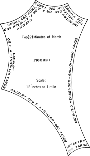
Military sketches are of three kinds:
- Position sketches, Fig. 1;
- Outpost sketches;
- Road sketches.
All kinds of military sketches are intended to give a military commander detailed information of the ground to be operated over, when this is not given by the existing maps, or when there are no maps of the area.
The general methods of sketching are:
(1) The location of points by intersection.
(2) The location of points by resection.
1879. Location of points by intersection. To locate a point by intersection proceed as follows: Set up, level and orient the sketching board (Par. 1872), at A, Fig. 1. The board is said to be oriented when the needle is parallel to the sides of the compass trough of the drawing board, Fig 2. (At every station the needle must have this position, so that every line on the sketch will be parallel to the corresponding line or direction on the ground.) Assume a point (A) on the paper, Fig. 1 Y, in such a position that the ground to be sketched will fall on the sheet. Lay the ruler on the board and point it to the desired point (C), all the while keeping the edge of the ruler on the point (A), Fig. 1 Y. Draw an indefinite line along the edge. Now move to (B), Fig. 1 X, plotted on the map in (b), Fig. 1 X, and having set up, leveled and oriented as at (A), Fig. 1 Y, sight toward (C) as before. The intersection (crossing) of the two lines locates (C) on the sketch at (c), Fig. 1 X.
1880. Locating points by resection. A sketcher at an unknown point may locate himself from two visible known points by setting up and orienting his sketching board. He then places his alidade (ruler) so that it points at one of the known points, keeping the edge of the alidade touching the corresponding point on the sketch. He then draws a ray (line) from the point toward his eye. He repeats the performance with the other visible known point and its location on the map. The point where the rays intersect is his location. This method is called resection. However, local attractions for the compass greatly affect this method.
1881. The location of points by traversing. To locate a point by traversing is done as follows: With the board set up, leveled and oriented at A, Fig. 1 Y, as above, draw a line in the direction of the desired point B, Fig. 1 X, and then move to B, counting strides, keeping record of them with a tally register, Fig. 3, if one is available. Set up the board at B, Fig. 1 X, and orient it by laying the ruler along the line (a)-(b), Fig. 1 X, and moving the board until the ruler is directed toward A, Fig. 1 Y, on the ground; or else orient by the needle as at A. With the scale of the sketcher's strides on the ruler, lay off the number of strides found from A, Fig. 1 Y, to B, Fig. 1 X, and mark the point (b), Fig. 1 X. Other points, such as C, D, etc., would be located in the same way.
1882. The determination of the heights of hills, shapes of the ground, etc., by contours. To draw in contours on a sketch, the following steps are necessary:
(a) From the known or assumed elevation of a located station as A, Fig. 1 Y, (elevation 890), the elevations of all hill tops, stream junctures, stream sources, etc, are determined.
(b) Having found the elevations of these critical points the contours are put in by spacing them so as to show the slope of the ground along each line such as (a)-(b), (a)-(c), etc., Fig. 1 Y, as these slopes actually are on the ground.
| (Tally Register)—Fig. 3 | (Clinometer)—Fig. 4 |
To find the elevation of any point, say C (shown on sketch as c), proceed as follows:
Read the vertical angle with slope board, Fig. 2, or with a clinometer, Fig. 4. Suppose this is found to be 2 degrees; lay the scale of M. D.[22] (ruler, Fig. 2) along (a)-(c), Fig. 1 Y, and note the number of divisions of -2 degrees (minus 2°) between (a) and (c). Suppose there are found to be 51/2 divisions; then, since each division is 10 feet, the total height of A above C is 55 feet (51/2 × 10). C is therefore 835 ft. elev. which is written at (c), Fig. 1 Y. Now looking at the ground along A-C, suppose you find it to be a very decided concave (hollowed out) slope, nearly flat at the bottom and steep at the top. There are to be placed in this space (a)-(c), Fig. 1 Y, contours 890, 880, 870, 860 and 850, and they would be spaced close at the top and far apart near (c), Fig. 1 Y, to give a true idea of the slope.
The above is the entire principle of contouring in making sketches and if thoroughly learned by careful repetition under different conditions, will enable the student to soon be able to carry the contours with the horizontal locations.
1883. In all maps that are to be contoured some plane, called the datum plane, must be used to which all contours are referred. This plane is usually mean sea level and the contours are numbered from this plane upward, all heights being elevations above mean sea level.
In a particular locality that is to be sketched there is generally some point the elevation of which is known. These points may be bench marks of a survey, elevation of a railroad station above sea level, etc. By using such points as the reference point for contours the proper elevations above sea level will be shown.
In case no point of known elevation is at hand the elevation of some point will have to be assumed and the contours referred to it.
Skill in contouring comes only with practice but by the use of expedients a fairly accurate contoured map can be made. In contouring an area the stream lines and ravines form a framework or skeleton on which the contours are hung more or less like a cobweb. These lines are accurately mapped and their slopes determined and the contours are then sketched in.
If the sketcher desires he may omit determining the slopes of the stream lines and instead determine the elevations of a number of critical points (points where the slope changes) in the area and then draw in the contours remembering that contours bulge downward on slopes and upward on streams lines and ravines.
If time permits both the slopes of the stream lines and the elevation of the critical points may be determined and the resulting sketch will gain in accuracy.
Figs. 5, 6, 7, 8, and 9 show these methods of determining and sketching in contours.
1884. Form lines. It frequently happens that a sketch must be made very hastily and time will not permit of contouring. In this case form lines are used. These lines are exactly like contours except that the elevations and forms of the hills and depressions which they represent are estimated and the sketcher draws the form lines in to indicate the varying forms of the ground as he sees it.
1885. Scales. The Army Regulations prescribe a uniform system of scales and contour intervals for military maps, as follows:
Road sketches and extended positions; scale 3 inches to a mile, vertical (or contour) interval, 20 feet.
Position or outpost sketches; scale 6 inches to a mile, vertical (or contour) interval, 10 feet.
This uniform system is a great help in sketching as a given map distance, Par. 1867a, represents the same degree of slope for both the 3 inch to the mile or the 6 inch to the mile scale. The map distances once learned can be applied to a map of either scale and this is of great value in sketching.
Construction of Working Scales
1886. Working scale. A working scale is a scale used in making a map. It may be a scale for paces or strides or revolutions of a wheel.
1887. Length of pace. The length of a man's pace at a natural walk is about 30 inches, varying somewhat in different men. Each man must determine his own length of pace by walking several times over a known distance. In doing this be sure to take a natural pace. When you know your length of pace you merely count your paces in going over a distance and a simple multiplication of paces by length of pace gives your distance in inches.
In going up and down slopes one's pace varies. On level ground careful pacing will give you distances correct to within 3% or less.
The following tables give length of pace on slopes of 5 degrees to 30 degrees, corresponding to a normal pace on a level of 30.4 inches:
| Slopes | 0° | 5° | 10° | 15° | 20° | 25° | 30° |
|---|---|---|---|---|---|---|---|
| Length of step ascending | 30.4 | 27.6 | 24.4 | 22.1 | 19.7 | 17.8 | 15.0 |
| Length of step descending | 30.4 | 29.2 | 28.3 | 27.6 | 26.4 | 23.6 | 19.7 |
For the same person, the length of step decreases as he becomes tired. To overcome this, ascertain the length of pace when fresh and when tired and use the first scale in the morning and the latter in the afternoon.
The result of the shortening of the pace due to fatigue or going over a slope, is to make the map larger than it should be for a given scale. This is apparent when we consider that we take more paces in covering a given distance than we would were it on a horizontal plane and we were taking our normal pace.
In going up or down a slope of 3 or 4 we actually walk 5 units, but cover only 4 in a horizontal direction. Therefore, we must make allowance when pacing slopes.
In counting paces count each foot as it strikes. In counting strides count only 1 foot as it strikes. A stride is two paces.
In practice it has been found that the scale of strides is far more satisfactory than a scale of paces.
1888. How to make a scale of paces. Having determined the length of our pace, any one of the following three methods may be used in making a working scale:
1st method. The so-called "One thousand unit rule" method is as follows:
Multiply the R. F. (representative fraction) by the number of inches in the unit of measure multiplied by 1000; the result will be the length of line in inches necessary to show 1000 units.
For example, let us suppose that we desire a graphic scale showing 1000 yards, the scale of the map being 3 inches equal 1 mile:
Multiply 1/21120 (R. F.) by 36 (36 inches in 1 yard, the unit of measure) by 1000,—that is,
(1/21120) × 36 × 1000 = 36000/21120 = 1.7046 inches.
Therefore, a line or graphic scale 1.7 inches in length will represent 1000 yards.
If we desire a working scale of paces at 3 inches to the mile, and we have determined that our pace is 31 inches long, we would have (1/21120) × 31 × 1000 = 31000/21120 = 1.467 inches.
We can now lay off this distance and divide it into ten equal parts, and each will give us a 100-pace division.
2nd method. Lay off 100 yards; ascertain how many of your paces are necessary to cover this distance; multiply R. F. by 7,200,000, and divide by the number of paces you take in going 100 yards. The result will be the length of line in inches which will show 2000 of your paces.
3rd method. Construct a scale of convenient length, about 6 inches, as described in Par. 1863, to read in the units you intend to measure your distance with (your stride, pace, stride of a horse, etc.), to the scale on which you intend to make your sketch.
For example, suppose your stride is 66 inches long (33 inch pace) and you wish to make a sketch on a scale of 3 inches = 1 mile. The R. F. of this scale is 3 inches/1 mile = 3 inches/63360 inches = 1/21120. That is 1 inch on your sketch is to represent 21120 inches on the ground. As you intend to measure your ground distances by counting your strides of 66 inches length, 1 inch on the sketch will represent as many of your strides on the ground as 66 is contained into 21120 = 320 strides. For convenience in sketching you wish to make your scale about 6 inches long. Since 1 inch represents 320 strides, 6 inches will represent 6 × 320 = 1,920 strides. As this is an odd number, difficult to divide into convenient subdivisions of hundreds, fifties, etc., construct your scale to represent 2,000 strides, which will give it a length slightly in excess of 6 inches—6.25. Lay off this length and divide it into ten main divisions of 200 strides each, and subdivide these into 50 stride divisions as explained in Par. 1862.
1889. Position sketching. The following are the instruments used in position sketching:
- Drawing board with attached compass (Fig. 2);
- Loose ruler, on board (Fig. 2);
- Rough tripod or camera tripod;
- Scale of M. D.'s (shown on ruler, Fig. 2);
- Scale of sketchers, strides or paces (at six inches to one mile), on ruler;
- Clinometer (not necessary if board has slope board, Fig. 6);
- Scale of hundreds of yards shown on ruler;
- Scale of paces.
Methods to be used
(1) Select a base line,—that is, a central line 1/4 to 1/2 mile long in the area to be sketched. It should have at its ends some plainly marked objects, such as telegraph poles, trees, corners of buildings, etc., and from its ends, and intermediate points, a good view of the area should be possible. The base line selected should be capable of being measured.
(2) Set up, level and orient the drawing board at one end of the base (A), Fig. 1, Y, for example. Draw a meridian on the sheet parallel to the position of the magnetic needle. Assume a point (A), Fig. 1, Y, corresponding to the ground point (A), 890, on the sheet, in such a position that the area to be sketched will lie on the sheet.
(3) Sight at hilltops, stream junctures, stream heads, etc., to begin the locations of these points by intersection, labelling each ray so as to be able to identify it later.
(4) Traverse to (b) and complete the locations by intersection as previously explained. If the base line is not accurately measured, the map will be correct within itself in all of its proportions, but its scale will not necessarily be the scale desired.
(5) Draw the details of the country between A and B and in the vicinity of this line, using the conventional signs for roads, houses, etc.
(6) The lines from station (b), Fig. 1, X, to any of the other located points may now be used as a new base line to carry the work over additional area.
(7) In case parts of the area are not visible from a base line, these parts are located by traversing as before explained.
(8) Having learned by several repetitions the above steps, the sketcher will then combine contouring with his horizontal locations.
1890. Outpost sketching. The same instruments are used as in position sketching, and so are the methods the same, except that the sketcher cannot advance beyond the outpost line, toward the supposed position of the enemy. It is often possible to select a measurable base line well in rear of the line of observation,—for instance, along the line of resistance. Secondary base lines may then be taken on or near the line of observation, from the extremities of which additional base lines may be selected, if necessary, and points toward the enemy's position located by intersection. Details are sketched in as in position sketching. For obvious reasons, no traversing should be done along the line of observation.
1891. Road sketching. The following are the instruments used in road sketching:
- Drawing board or sketching case;
- Loose ruler;
- Scale of strides, or paces, if made dismounted; scale of time trotting or walking, if mounted;
- Scale of hundreds of yards, at three inches to 1 mile;
- Scale of M. D.'s;
- Slope board (if clinometer is not available).
Methods to be used
(1) At station 1, Fig. 10, orient the board as described in par. 1872, holding the board in the hands, in front of the body of the sketcher, who faces toward station 2.